The Interpolation
Process
By: Philip Wyatt
A look at
the fundamentals of grid surface generation
There are
many advantages to taking spatial data beyond a purely descriptive display
method, such as the thematic mapping of points using colors or proportionally
sized symbols. Modeling and interpolation software provide the means necessary
to process and display data in a new derivative form. However, you cannot take
full advantage of this evolving technology without a good fundamental
understanding of grid surface generation. While these examples were created
using MapInfo
Professional with Vertical
Mapper, the principles are applicable no matter what software you use.
Imagine
you had collected 1,000 census data points in 1998 from a fixed area. In 1999
you collected 2,000 points over the same region, in different locations. How
will you compare the 1999 and 1998 points to see increasing or decreasing trends?
It is not possible to use simple database math to subtract one year from the
other because the tables do not line up. The solution is to convert both point
files into continuous grid layers that can easily be overlaid and compared.
Point files are converted into grids by interpolation. It is my hope to take
some of the mystery out of this operation, pique your interest in grid mapping
and show off some features of surface generation software in the process.
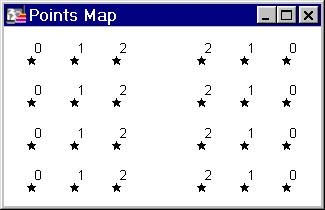
Let us
start with a simple point file. 24 points are arranged in a regular fashion
with attribute values ranging from 0 to 2 as shown below.
The
attribute can be as varied as a dollar value or the signal strength level of a
cellular phone. As long as it is numeric it can be represented in 3D form, as
depicted below. In fact, the image is actually a rendered grid. The grid was
generated using IDW interpolation, sampling only one data point (to exactly honor
the data values), using a very small display radius equal to the width of a
single column. Rendering this sort of sparse grid creates a unique thematic map
akin to a 3D bar chart.
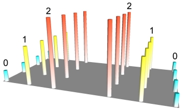
Point values represented in 3D space
Of course
the main reason for using grids is to build a continuous surface that connects
the data points in space, effectively removing gaps in the representation of
data and facilitating comparison of datasets.
To fully
take advantage of this technology one must have a clear mental picture of what
grid surfaces are, what type of surface best represents the intervening area
between known data points, and which interpolation technique must be used to
generate an appropriate surface. While I cannot answer all those questions in
this article, I can give you a taste of what's possible and start you thinking
in 3D.
There are
two properties that must be determined before choosing an appropriate
interpolator for a dataset:
- How reproducible is the
data (a function of the collection and analysis techniques)?
- Does the data point
represent only a value at that point in space, such as an elevation point,
or does it represent a property from a wider area such as an enumeration
area centroid?
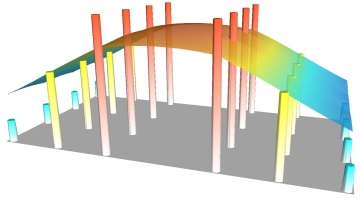
If our 3D point map represented a demographic variable such as average
household income then a constant natural neighbor (NN) surface, as shown below,
might be a reasonable approximation.
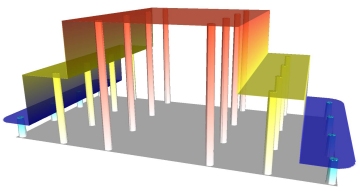
Natural neighbor interpolation, constant mode
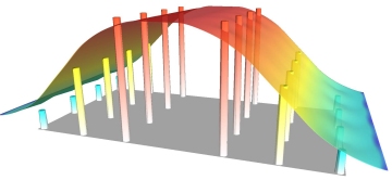
If the
rate of change between regions surrounding a point is too abrupt, then it is
possible to adjust the Natural Neighbor interpolator to make a gradual sloped
surface between the points. This includes minor smoothing and limiting the
maximum and minimum values of the surface so that no part of the grid has a
value beyond the range of the original point data.
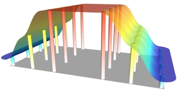
Natural neighbor interpolation,
using slope but limiting over/undershoot
If the
data points represent elevation values of a buried bedrock surface that acts as
an oil or gas trap, then we may require the interpolated grid surface to curve
above or below the range of the sampled data points. It isn't possible to
guarantee that exploratory drilling will intersect the apex of the dome and
thus it is necessary to model this curvature as shown below.
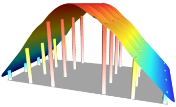
Natural neighbor interpolation,
using slope and allowing over/undershoot
Understanding
the reproducibility of the data determines whether or not we need the
interpolated surface to exactly pass through the data points or we require a
surface which simply represents the general trend. Inverse distance weighting
is one interpolation method that performs a moving average or
"smoothing" of the data. For instance, many bulk soil chemistry
analyses produce fairly reproducible results. The example below shows a
slightly smoothed surface generated by Inverse Distance Weighting. The high and
low data points are not exactly honored.
Inverse Distance Weighting with some smoothing
On the
other hand, analyzing for gold requires sieving out a very small amount of
material from the soil sample and dissolving it in acid and vaporizing it in
the flame of an atomic absorption spectrometer. Not surprisingly, if you return
to the area where the soil sample was taken, dig another hole and repeat the
process, chances are that it will yield a rather different result (the
"nugget" effect). In this case, it would be appropriate to represent
the data points with a grid which heavily smoothes the data, showing the
general trend but masking the irreproducible results. Interpolation by kriging
is one such method, while it can also be used as an exact interpolator. The
example below uses kriging with an option to smooth the data heavily.
Kriging with heavy smoothing
So there it is. Build a simple data set and begin experimenting. Vertical
Mapper has many grid generation and visualization tools that make it easy
and intriguing to explore and understand the effect of small changes in
interpolation settings. A whole new world of benefits awaits those who can
visualize their data as a 3D surface!