TIME INTEGRATION

Constitutive models are integrated using explicit adaptive integration scheme with local substepping. The constitutive model forms an ordinary differential equation of the form

$$\frac{dy}{dt}=f(t, y)$$

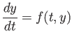
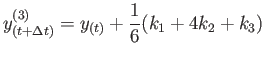
The equation is for finite time step size $\Delta t$ solved using the Runge-Kutta method. Solutions that correspond to the second- and third- order accuracy of Taylor series expansion are given by

$$y_{(t+\Delta t)}^{(2)}=y_{(t)}+k_2$$

$$y_{(t+\Delta t)}^{(3)}=y_{(t)}+\frac{1}{6}(k_1+4 k_2 + k_3)$$

where

$$k_1=\Delta t f\left(t, y_{(t)}\right)$$

$$k_2=\Delta t f\left(t+\frac{\Delta t}{2}, y_{(t)}+\frac{k_1}{2}\right)$$

$$k_3=\Delta t f\left(t+\Delta t, y_{(t)}-k_1+2 k_2\right)$$

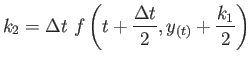
The accuracy of the solution is estimated following Fehlberg as the difference between the second- and third- order solutions. The time step size $\Delta t$ is accepted, if

$$err=\left\Vert y_{(t+\Delta t)}^{(3)}-y_{(t+\Delta t)}^{(2)}\right\Vert < TOL$$

where $TOL$ is a prescribed error tolerance. If the step-size $\Delta t$ is accepted, $y_{(t+\Delta t)}^{(3)}$ is considered as a solution for the given time step and the new time step size $\Delta t^n$ is estimated according to Hull

$$\Delta t^n={\rm min}\left[4\Delta t, 0.9 \Delta t \left(\frac{TOL}{err}\right)^{1/3}\right]$$

If the step-size $\Delta t$ is not accepted, the step is re-computed with new time step size

$$\Delta t^n={\rm max}\left[\frac{\Delta t}{4}, 0.9 \Delta t \left(\frac{TOL}{err}\right)^{1/3}\right]$$

In the case the prescribed minimum time step size or the prescribed maximum number of time substeps is reached, the finite element program is asked to reject the current step and to decrease the size of the global time step.