 Part 3: Biological Sequence Phylogenies
For computing phylogenetic trees we are going to use PHYLIP, FastTree, IQ-TREE and MrBayes.
For the visualization of trees, we are going to use FigTree.
The question of today - Is the guinea-pig a rodent?
While this might sound silly today, in the 90s this was a Nature journal-level debate that was ultimately resolved by Bayesian inference in 2001. We are going to replicate this issue by using different tree-inference methods and discuss their disadvantages. Let's first start with the simplest, distance methods.
Models for phylogenies
The methods used in the 90's have their drawbacks, which stems from computational limitations at the time of their conception (your phones are probably faster). For comparison, we are also going to use more advanced methods of (approximate) maximum likelihood and Bayesian inference.
Let us have a look at some parameters behind the scene first.
Selected models of DNA evolution often used in molecular phylogenetics
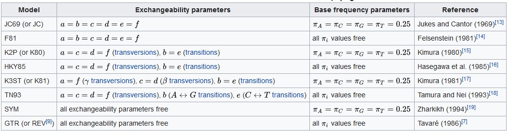
For each character (site in alignment), the probability of its existence is governed by two major variables, the frequency of this character in biological molecules, (Base frequency parameters in the table above) and the frequency of its change to another one (Exchangeability parameters in the table above). As is apparent from the DNA evolution models, each of them employs different parameter estimation, ranging from fixed frequencies for base exchange and base frequency (Jukes-Cantor or JC) to a complete freedom in the estimation of these parameters (Generalized Time Reversible or GTR).
Then again, each character in an alignment might mutate at a different rate (e.g. there are steric limitations for some amino acids to mutate in a given protein, and so its gene is conserved accordingly). To reflect this, algorithms invoke another function (gamma = Γ) that defines several (usually 4) discrete categories based on mutation rates and then assigns each alignment character a likelihood value based on the probabilities of belonging to any of these categories.
Model choice - Distance
With more parameters, tree inference accommodates better the biological substitution processes, but the variability and deviation of each parameter values also increases.
This leads to an increased influence of randomness, especially with large number of taxa (as a rule of thumb, there should be at least as many informative positions in the alignment as there are sequences).
Distance methods are typically prone to such errors and an optimal model should be chosen in each case.
Many people suggested different ways to choose the most optimal models. Here are two examples:
According to Nei and Kumar:
If the computed Jukes-Cantor distance (d) is < 0.05, this is an appropriate model and gamma correction is not necessary.
If d is higher, there is a large difference between transitions and transversions (R>5), and sequences are long enough, 2-parametric Kimura or gamma-correction is appropriate. For short alignments and/or large number of taxa, use Jukes-Cantor.
Furthermore, Swoford et al.:
Complex models are appropriate when the number of positions is >2000.
LogDet distance is a very general, low-deviation approach robust against variations in nucleotide composition. However, it is susceptible to different substitution rates across codon sites, which cannot be corrected for. It does not support invariable sites, either and they need to be removed.
To summarize, chosing the right model is critical for your dataset. Choosing a too complex model for your alignment, leads to overparameterization, however, choosing a very simplistic model for a complex dataset leads to under-parameterization. Both mistakes, lead to poor resolution of the phylogenetic trees.
If possible, multiple models should be applied and their results compared. However, for branch length calculation, always use more accurate, complex models.
In Maximum Likehood methods, algorithms often automatically employ likelihood ratio tests (LRT). These determine, how much more likely is the tree based on a complex model compared to a simple model.
Other considerations - Gaps
Gaps that remain after alignment trimming are treated differently in various programs. Mostly they are considered as unknowns and disregarded in the phylogenetic inference, but sometimes they might be considered as bearing phylogenetic signal. Compare gapped and gapless alignments if in doubt.
Data for today:
Alignments:
Reference tree:
Let's trim the alignments, export them as strict phylip format in Aliview, and compare their content. Make a working directory for today's exercises to keep your files organized.
mkdir moltax
cd moltax
ls #make sure your files are here!
bmge -i INFILE -of OUTFILE -t AA -g 0.2 -h 1.0
trimal -in INFILE -out OUTFILE -fasta -gt 0.8
Check the tree files as well, opening them in FigTree and a notepad as well. What are the main differences?
Distance methods - Neighboor joining.
For this we will use PHYLIP. This is a rather old program, which we use to demonstrate the various steps employed to obtain a phylogeny.
1. To check if PHYLIP is installed and working on your computer, type in the terminal:
phylip
A list of available functions should be listed
For this we will use the mammalian nucleotide ATP7A fasta. Open your trimmed file in AliView to convert it to a strict PHYLIP file if you haven't done so.
2. First we make a new directory called phylip
mkdir phylip
3. Now we enter this directory
cd phylip
4. Copy the PHYLIP alignment file to the current directory
5. Let's make a copy of the alignment file and name it infile
cp ALIGNMENTFILE infile
When your file is called
infile, phylip will pick it up as the default input file and will automatically work on it.
6. We will use seqboot to create a boostrap file
phylip seqboot
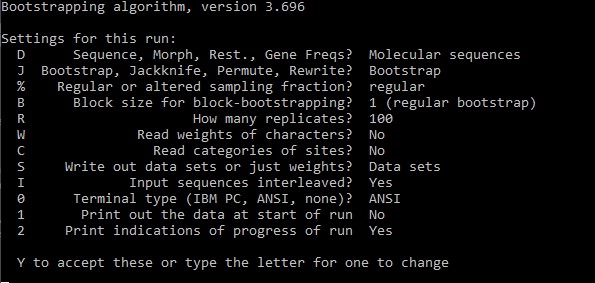
You can press R and write the number of replicates. We will compute 100 replicates for now.
After you are satisfied with the settings press Y to confirm and phylip will compute the permutated alignments. These are written in outfile.
The bootstrap file is a randomized set of the original data.
7. After computation, rename the outfile to infile for the next step.
mv outfile infile
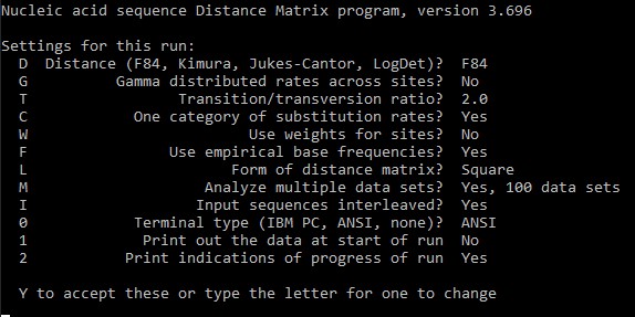
8. Now we will compute the distances for each bootstrap.
phylip dnadist OR protdist ####one OR another, depending on your datafile
9. Phylip already used infile as your input. We need to instruct the program that we have multiple replicates in this file. For this press M and then you will be asked what type of replicates, we select D because we have Data sets and then we type in the number of replicates.
After computation, we will have the results in outfile. Again let's rename first the infile and then rename the outfile to infile
mv infile ALIGNMENT_bootstrapmv outfile infile
10. Let's start the neighbor-joining of each bootstrap.
phylip neighbor
11. Phylip already used infile as your input. We need to instruct the program that we have multiple replicates in this file. For this, press M and then we type in the number of replicates.
This time the software made for you two files. One is the outfile and the other is the outtree. We will use the outtree file for the next step.
12. We rename the outfile and the outree file as well as the infile.
mv infile ALIGNMENT_distmv outfile ALIGNMENT_nj_outfilemv outtree intree
13. Now we build a consensus tree using consense
phylip consense
The file named outtree now contains our consensus NJ tree with support values. We will check it with FigTree. Compare to the reference tree.
Similarly, one would do maximum parsimony with the
dnapars/dnapenny/protpars.
Maximum likelihood methods - FastTree
FastTree is usually the method of choice for large number of taxons
The algorithm is an approximately-ML process designed for up to a million sequences and is said to be 100-1,000 times faster than RAxML with a slightly worse accuracy.
First, a rough topology is obtained by heuristic neighbor-joining. Then, the length of the tree is shortened by nearest-neighbor rearrangements (NNI) and subtree-prune-regrafting (SPR). Finally, the tree is optimized by ML.
The main limitation of FastTree is the fact that there is just a few available models.
For DNA: Jukes-Cantor and GTR
- For protein: JTT and WAG
FastTree accepts as input FASTA and PHYLIP alignments.
To run FastTree:
fasttree PROTINFILE > OUTTREE #protein defaultfasttree -nt NUCLINFILE > OUTTREE #for nucleotide
The resulting trees contain likelihood values by default.
Maximum likelihood methods - IQ-TREE and RAxML
Standard programs for phylogenetic analyses include RAxML and IQ-TREE.
These algorithms start with a maximum parsimony tree, followed by NNIs/SPRs with all tree branches. If a better tree is found, the old one is replaced. The algorithms finish when they cannot find a better tree anymore.
Their performance is roughly comparable, although newer versions are improved (RAxML-NG and IQ-TREE2). IQ-TREE is highly automated and offers a lot of extra functions, including the most sophisticated protein models.
For our purpose we will use IQ-TREE.
Check the functionality of IQ-TREE:
iqtree -h
Note parameters:
-s input alignment in FASTA/Phylip/Nexus format-m model name / MFP (stands for ModelFinder Plus)-b/-B non-parametric / ultra-fast bootstrap-T num threads-merit likelihood parameter to decide upon (AIC/AICc/BIC)-msub restrict model search to AA models from specific sources (nuclear, mitochondrial, chloroplast or viral)
Let's use IQ-TREE to find the best fitting model for our current dataset. To run IQ-TREE best model finding mode, enter:
iqtree -m MF -s NUCLINFILE
Check which model was found to be the best. What is the difference between the chosen model and the Jukes-Cantor model?
Now finish the analysis by using the best model and ultrafast bootstrapping. In this case we have to rewrite previous results, which is why we need to use the -redo parameter:
iqtree -m MFP -redo -B 1000 -s NUCLINFILE
This time, the computation might have taken longer time than before. However, the ultra-fast method stops the analysis once finding a significantly better tree than the one it started with. For a more robust analysis one might consider non-parametric bootstraps.
Open the trees we have created so far in FigTree and compare their topologies. Do you see any differences? Now let us compare our results with analyses in protein space, which might be more suitable over larger evolutionary distances when nucleic acid characters become saturated with exchanges.
Exercise 1
Choose the best model according to the Akaike Information Criterion and compute the phylogeny from the primate 12S rDNA dataset.
Protein phylogeny methods - Maximum likelihood
In IQ-TREE the syntax for ML for protein data is very similar, only the models are different. One might also consider models specifically designed for proteins that have different evolutionary pressure, e.g. viral, transmembrane or mitochondrial matrices.
Exercise 2
Compute a ML phylogeny from the Mammalian ATP7A protein dataset.
What is the best model in this case? What is the best model for MrBayes?
Hint: use -mset parameter to identify the best model for MrBayes.
Protein phylogeny methods - Bayesian inference
For Bayesian inference, commonly used programs include MrBayes and PhyloBayes. The principles are similar to ML and more comprehensively explained in the manual of an older version of MrBayes. In brief, based on the a priori hypothesis on the tree topology under the assumed model, the algorithm evaluates the likelihood of observing the given data (i.e. the sequence alignment) and thus the posterior probability of that hypothesis. Inferring the likelihoods of all possible trees (hypotheses) is computationally demanding, which is why a workaround is implemented.
During the “tree space” exploration by the Markov chain Monte Carlo (MCMC) chains, certain topologies will occur at a frequency that is close to their posterior probability. Starting from a random tree, there are four MCMC chains in each of two parallel analyses, three are “hot” and looking for more divergent topologies to avoid being stuck at local likelihood optima. One chain is “cold” and collects (samples) the topologies. Under certain circumstances, the cold chain exchanges with a hot one, increasing sampling diversity. After a number of sampled generations, the results of the two parallel analyses are compared. If they reach convergence (i.e. the standard deviation of split frequencies of the chains is less than 0.01), the computation should be stopped. Then, the samples from the first 25% generations are discarded as burn-in (these are the trees from the initial tree space search), and a consensus is built from the rest.
The models available for Bayesian inference are somewhat different.
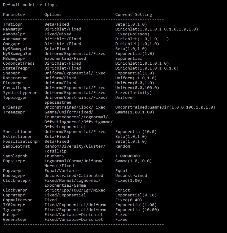
We will use mainly MrBayes. Type mb to start MrBayes, then to get help with model parameters type:
help lset
Look at the table at the bottom:
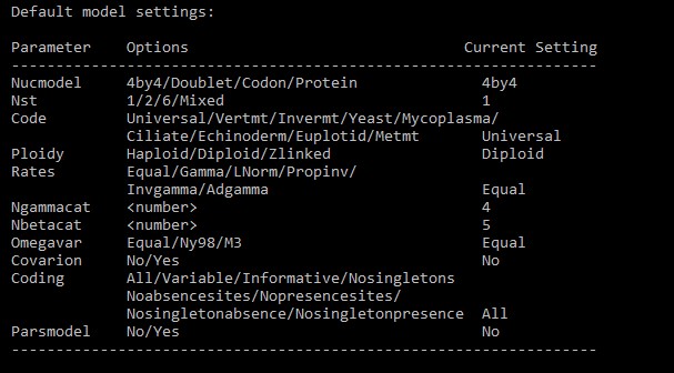
Nucmodel defines molecule type (4by4 for nucleotides, doublet for paired stem rDNA, codon for codon alignments, protein for proteins). Relevant for proteins are also Ngammacat (number of gamma categories) and Rates. Invgamma is a synonym for G4+I from IQ-TREE (four gamma categories plus invariant sites), so we can use this. MrBayes defines the covarion model for modelling heterogeneous substitution rates across tree branches.
To define prior probability distributions and substitution rates, check:
help prset
The most relevant parameter is Aamodelpr, which defines the substitution matrix. Set to mixed to analyse multiple rate matrices and choose the best, or set a fixed one by e.g. Aamodelpr=fixed(Jones).
In this course we will use MrBayes both locally (for demonstration and consensus tree computation) and online (for running the memory intense MCMC chains). The program accepts files in the NEXUS format.
Let's stop here with the theory and:
1. Export your Mammalian ATP7A protein FASTA as NEXUS in AliView;
2. Tweak the nexus output a little. Open the file in a text editor, change the FORMAT line as follows:
FORMAT DATATYPE=PROTEIN MISSING=-;
Then append the content below to define the so-called MrBayes data block at the end (replace OUTFILE with a desired output name, might be the same as the input). Change the model if needed.
BEGIN mrbayes;set autoclose=yes;log start filename = mrbayes.log.txt;prset aamodelpr=fixed(Jones);lset rates=gamma Ngammacat=4;mcmc ngen=1000 printfreq=100 samplefreq=100 nchains=2 savebrlens=yes filename=OUTFILE;log stop;quit;END;
Change the line break to Unix type if necessary and save. Type mb to start MrBayes.
Unix systems use a different line break symbol than Windows, which can cause issues. In your Notepad++, check this with Edit > EOL Conversion > UNIX Format.
To start your analysis, type in the terminal where you started MrBayes:
execute NEXUSFILE.nexus
You should see the analysis finish after 1000 generations (ngen=1000). When running properly, you would substantially increase sampling by replacing the mcmc parameters with something like:
ngen=1000000 printfreq=10000 diagnfreq=10000 samplefreq=1000 nchains=4
This would take several hours or days to finish, so we are providing the results here and here. Download the files to your working directory and unpack them using gzip:
gzip -d ATP7A_aa.Jones.run1.t.gz && gzip -d ATP7A_aa.Jones.run2.t.gz
To compute the consensus tree from our provided data, reopen the nexus file and append the content below. As OUTFILE, use the same prefix as for the MCMC chains. Replace the original MrBayes run parameters, or put the entire block into square brackets [ ] for future reference (i.e. put "[" before BEGIN and "]" after END;), which will "comment" this section and skip these steps. The consensus commands are:
BEGIN mrbayes;log start filename=OUTFILE.con.log replace;sumt filename=OUTFILE relburnin=yes burninfrac=0.25 contype=allcompat;END;
Now execute the file in the terminal where you started MrBayes:
execute NEXUSFILE.nexus
Note: You will get an error message if the analysis did not reach the specified number of MCMC generations, and "END;" was not appended to the runX.t files, closing the nexus data block. You can work around this by just writing END; to the end of both runX.t files yourself.
Open the resulting consensus tree (OUTFILE.con.tre) in FigTree and compare the topologies and the support values with the previous results.
To check if the burn-in was set properly, import the trace data into Excel or Tracer and plot the likelihood values against generations (LnL columns from the standard output) – they should reach a plateau value. You can quickly extract the first two columns using:
cut -f 1,2 ATP7A_aa.Jones.run1.p > likelihood.tsv