Introduction | Projection detection | Installation | Using the tool | Samples | Supported projections | References
Using the tool
Main controls
- Left mouse click: add control point.
- Right mouse click: delete the control point.
- Mouse wheel: Zoom in/out.
- Left mose drag: move the control point.
- Right mouse drag: dynamic shift of the map.
Control points
The analysis is based on the minimization of the squares of residuals between test points and projected reference points. The control points are collected by the user.
A pair of control points contains the control points on the analyzed map and on the reference map.
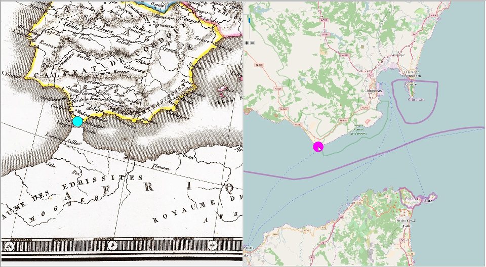
![]() symbol of the test point on the analyzed map,
symbol of the test point on the analyzed map,
![]() symbol of the reference point on Open Street Map.
symbol of the reference point on Open Street Map.
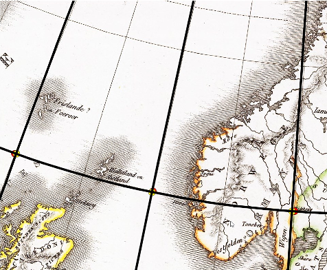
Control points located on the map items:
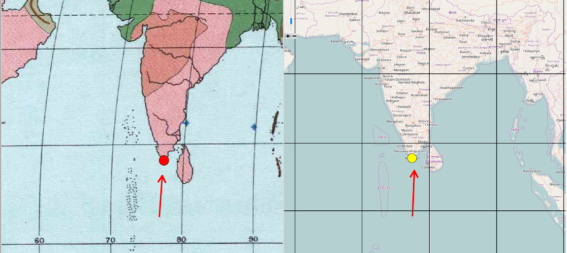
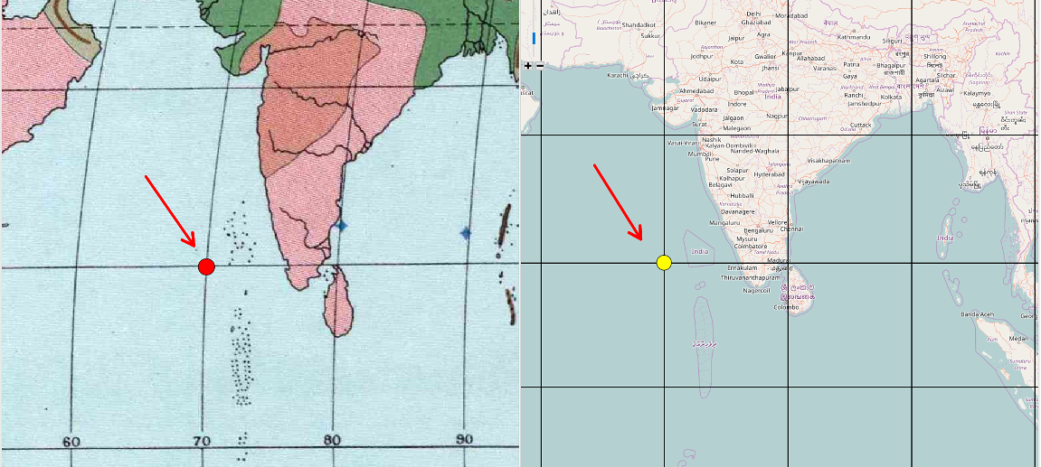
Control points located on the meridian/parallel intersection:
Properties of the control points
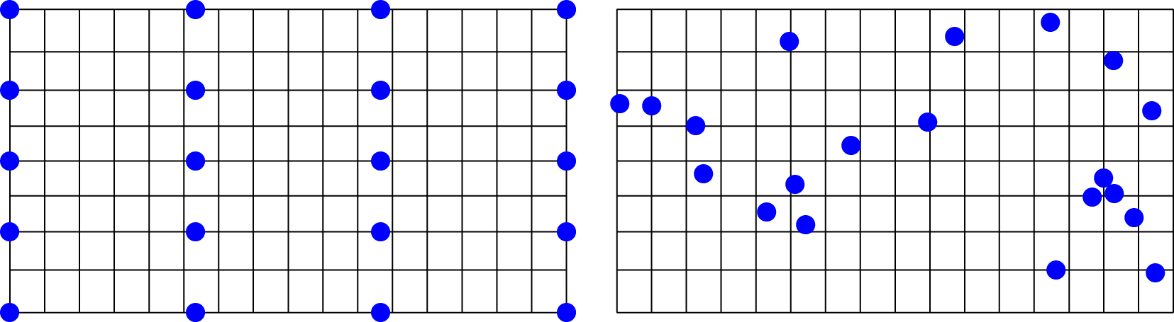
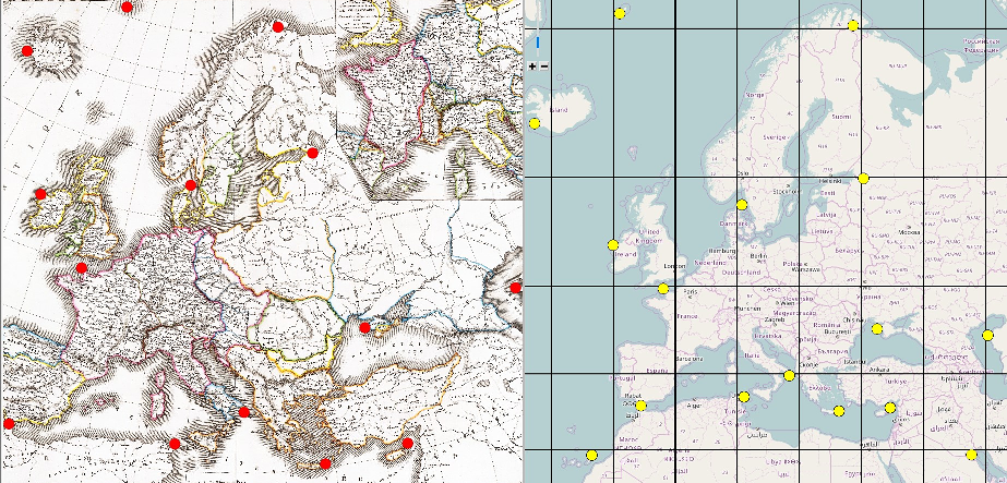
The proposed techniques are suitable for sets with approximately the same spatial density of features. On the boundaries of the analyzed region, in particular, it is necessary to place enough points.
- The uniform distribution of analyzed collected points on a map (grid, random set) is crucial.
- The estimated parameters fit well inside the convex hull of the analyzed set; noextrapolation of results outside the analyzed set is supported.
- The proper estimation of parameters on the boundary of the map, the analyzed features should be collected at the margins of the map.
- For the small-scale maps 5 points are sufficient, for the medium-scale maps 10 points are recommended, but for the large-scale maps 15-20 points may be required.
- For early maps, the graticule is significantly more accurate than the map content. Placing control points in the meridian and parallel intersections brings lower residuals between the original and reconstucted graticule.
The recommended control point distributions:
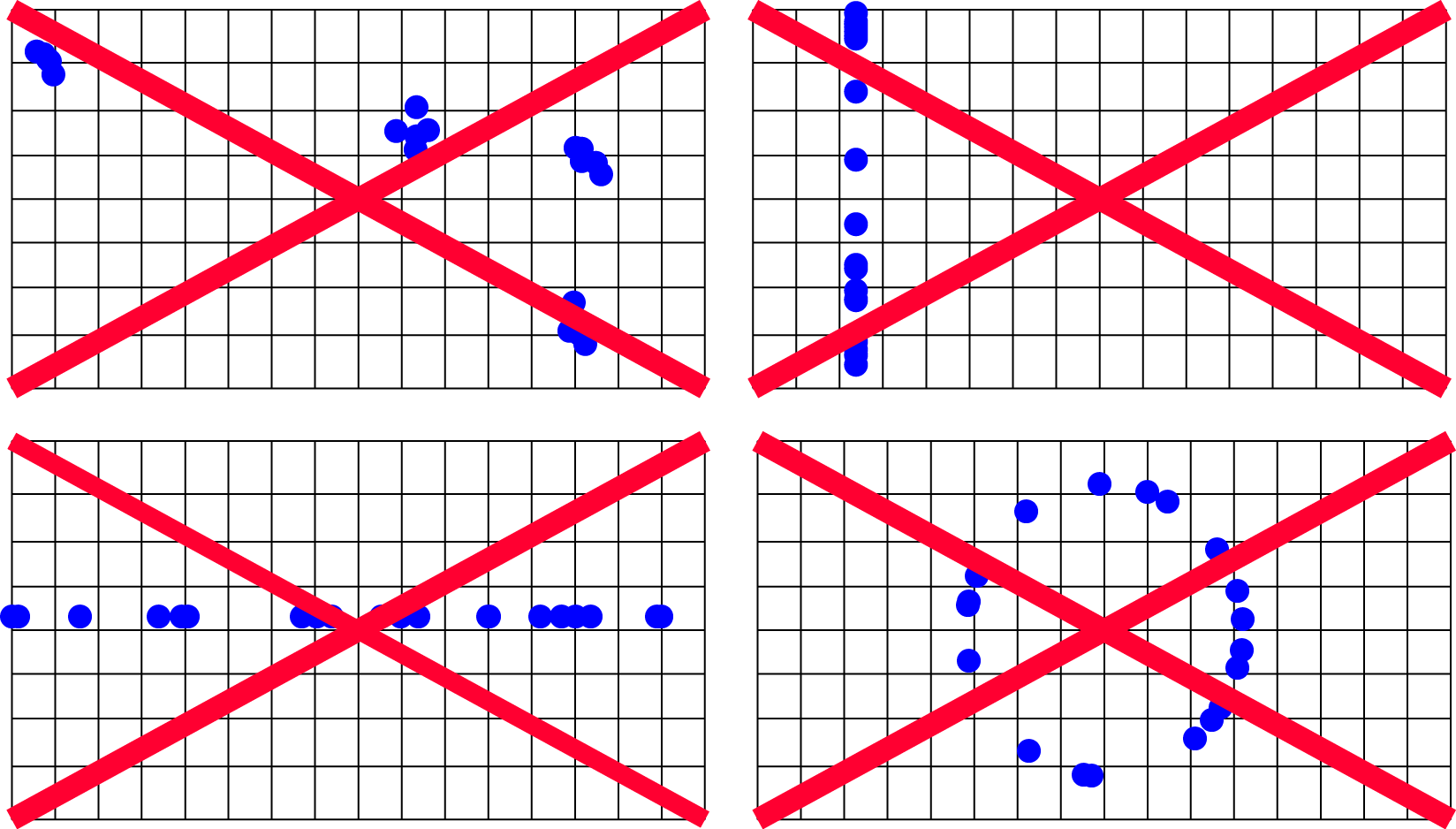
Not recommended point distributions:
Our algorithm performs recursive splitting of an edge depending on its geometric complexity and significance. The splitting criterion is calculated for each detected edge of the building. It is based on the calculation of standard deviation σ, that minimizes the sum of the squares of the points distances from the regression line; the variance of the residuals is the minimum possible. The regression line is oriented in accordance with one edge of the smallest area enclosing rectangle, it is parallel to this edge. The regression line also passes through the center of gravity of the set of points.
Analyze projection of the early map
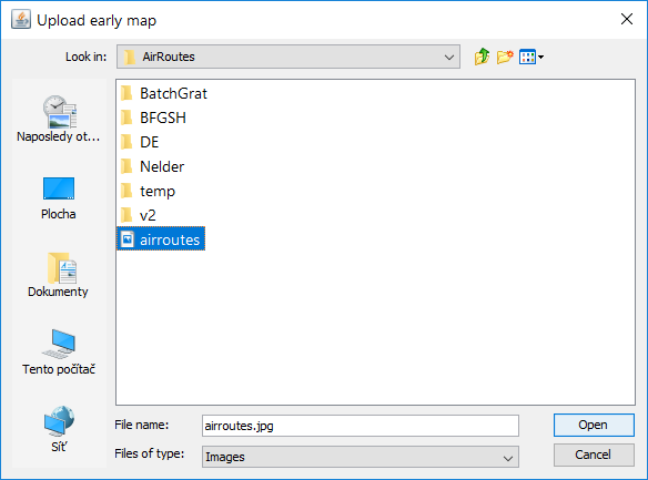
Step1: Import early map
The existing early map can be imported from a file. For successfull import, the file can not exceed 50 MB. The following graphic formats are supprted:
- JPG - Joint Photographic Expert Group,
- PNG - Portable Network Graphics,
- GIF - Graphics Interchange program.
To import early map file do the following steps:
- Click File in the menu, and select the Import map item. Alternately, click on the icon.
- In the dialog window Upload early map select the graphic file.
Step2: Collect control points
A pair of control points is represented by the control point on the analyzed map and the control point on the reference map. Regardless the order in which control points are collected (analyzed map first and reference map second or vice versa) a pair will be added to the list.
- Using mouse wheel or Zoom in tool zoom the map and find a feature on the map suitable for the analysis. Check its depiction on the reference map.
- In the toolbar, left-click on the Add control points tool .
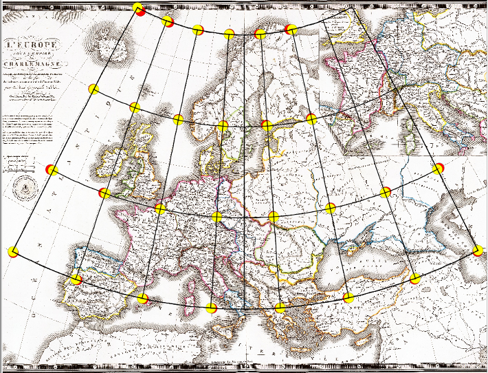
- Move the cursor above the desired control point and press the left mouse button. Above the early map, the red control point mark. Analogously, the yellow control point mark appears.
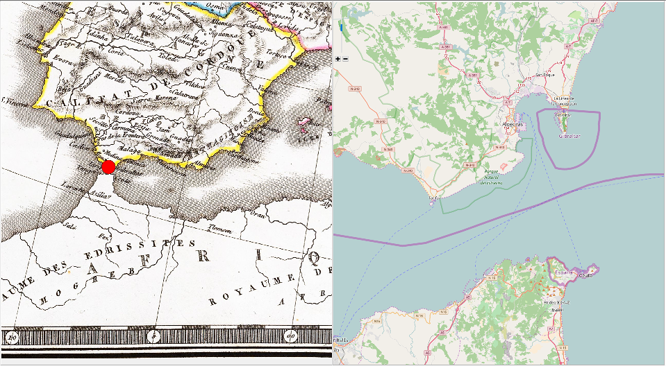
- Move the cursor above the corresponding point on the second map and press the left mouse button. The control point mark appears
- Repeat these steps until all control points are collected.
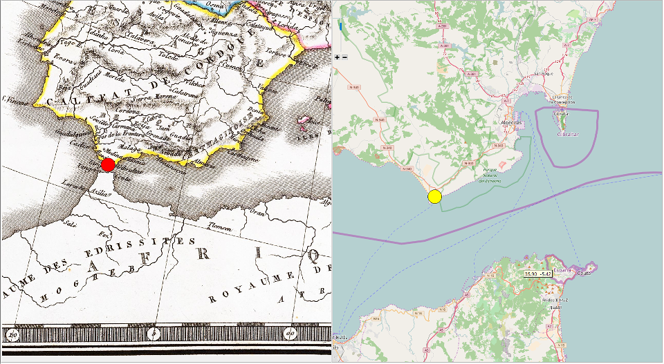
Move control points
- Move the cursor above the desired control point, the pair of control points highlights. On the reference map, its feographic coordinates are displayed.

- Dragging the mouse move the point to a destination position.
Step 3: Selection of the detection method
Before analysis it is necessary to select the detection method.
- From the Combo Box select the desired the detection method.

Alternately, click in the Analysis menu, and choose the detection method.
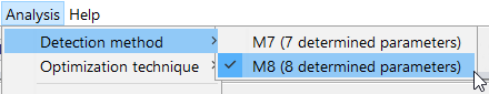
- Click in selected item, the highlighted method is checked and set as active.
M7 is recommended for the unrotated maps; this option is suitable for most situations. M8 achieves the best results for the rotated maps (a map rotation α is involved). This is typical for situations, when the map is incorrectly placed into the scanner or has a switched orientation on the page. Although M8 brings lower residuals, some solutions might be artificial and represent only a geometric construct not used by the cartographer.
Step 4: Selection of the optimization technique
Subsequently, the optimization technique needs to be chosen.
- From the Combo Box select the desired the optimization technique.
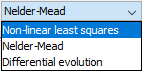
Alternately, click in the Analysis menu, and choose the optimization technique.
- Click in selected item, the highlighted technique is checked and set as active.
The NLS method represents the convex optimization technique which does not ensure the global minimum; only local minimum is found. The direct search technique, Nelder-Mead optimization, belongs to the global optimization methods. Due to small population, the global minimum may not be found. However, it is the fastest method. The differential evolution is the most efficient implemented technique performing a deep exploration of the search space. Unfortunately, it is also the slowest technique.
Step 5: Run analysis
Recall that at least five pairs of control points need to collected. Due to the time reason, do not use more than 30 control points. There are also several above mentioned recommendations on the control points that must be respected.
- Click on the
 button. Alternately, click in the Analysis menu, and choose the Analyze map item.
 - Depending on the amount of analyzed points, selected detection method and optimization technique, the results are evaluated within 10 seconds.
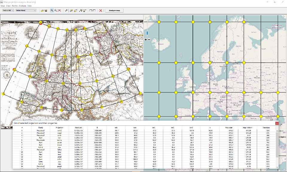
Step 6: Browse results
Let's look more closely at the results provided by the detectproj software.
Residuals. The residuals between the test and projected points can be found in the form List of control points form. The possible incorrectly placed control points can be found, moved, or rejected.
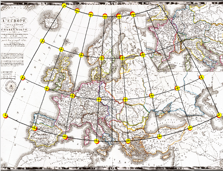
Reconstructed graticule. The reconstructed graticule is drawn over the analyzed. Depending on the early map, amount of control points, their accuracy, it provides a good fit. Ideally, the positional or shape discrepancies between the early map and reconstructed graticule should be less than the graphical accuracy of the map (0.1 mm) However, there might be some situations, when the results are not great.
Projected reference points. The reference points, drawn with the yellow map markers, projected using the best fit projection, are drawn over the analyzed map. In most situation there is a good fit between the test and projected reference points.
Vector of residuals. The vetors of residuals between the test and projected reference points are drawn over the analyzed map. Currently, they are visible only under magnification which indicates a good fit.
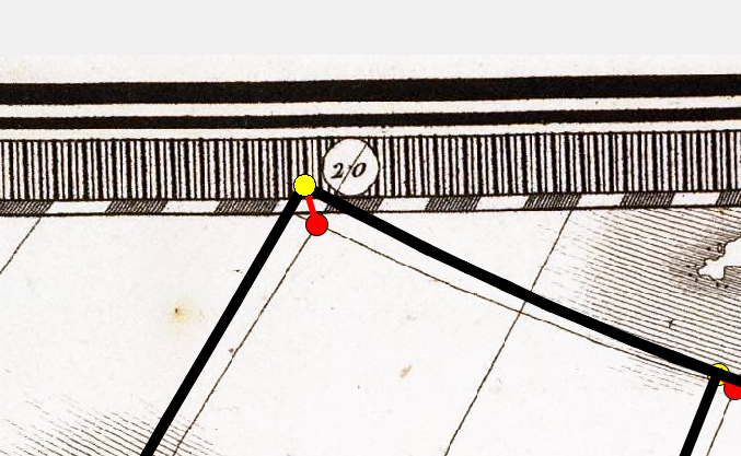
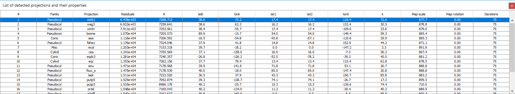
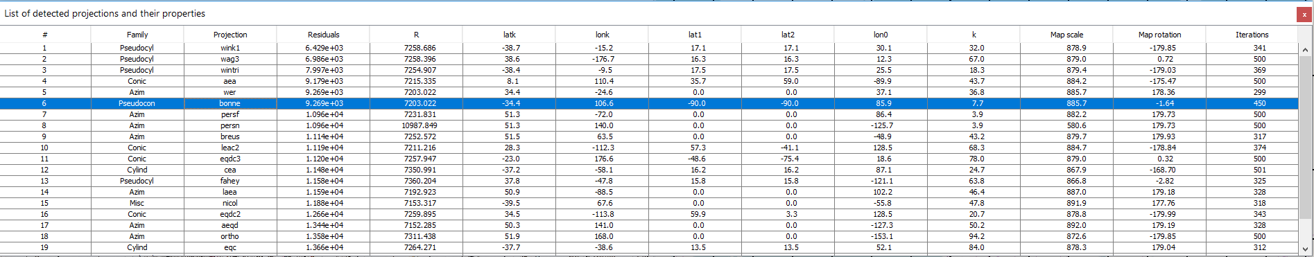
Table list of List of detected projections and properties
The table summarize results of 20 best-fit projections, their determined parameters as well as the parameters of the analyzed map.
Display results of different projections
After completing the analysis 20 candidate projections and their parametersare summarized in the table List of detected projections and properties. Currently, the resonstructed graticule, projected points and vector of residuals refer to the best-fit projection. To change the active projection do the following steps.
- Click on the
 button. Alternately, click in the Analysis menu, and choose the Show results item.
- Find the desired projection in the table List of detected projections and properties.
- In the table, click on the row and make the projection active; the table row which higlihts.
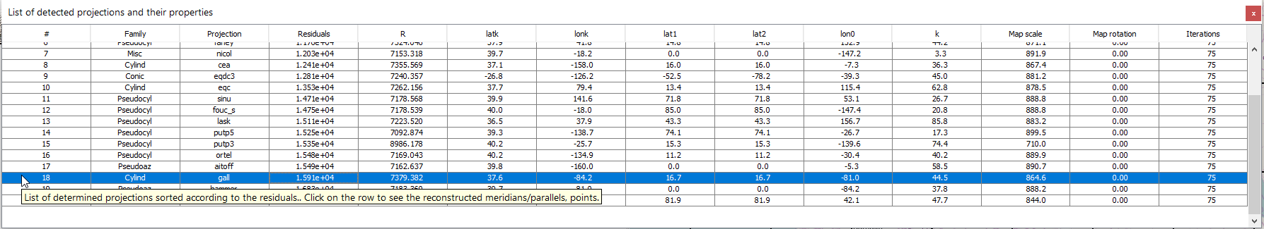
Subsequently, the reconstructed graticule, projected points and residuals refer to the active projection.
The differencies beteen candidate projections are not crucical. Sometimes, the possitional differencies are less than thegraphical accuracy of the map. For example, see the results between the Bonne projection (4th position, normal aspect).
and Gall projection (oblique aspect, 18th position).
Unlike the Bonne projection with the curved meridians, the Gall projection uses straight parallels.
Step 7: Export reconstructed graticule
The reconstructed graticule, test, and reference projected points can be extracted to the DXF file. It can be processed by CAD or GIS software. Any candidate projection from the List of detected projections and properties may be used to project the reference points and to create a graticule.
- Click on the click in the Analysis menu, and choose the Show results item.
- In the table, click on the row and make the projection active; the table row is higlighted.
- Click in the Map menu, and select the Export graticule item. Alternately, click on the icon.
- In the dialog window Export test points select the output DXF file.
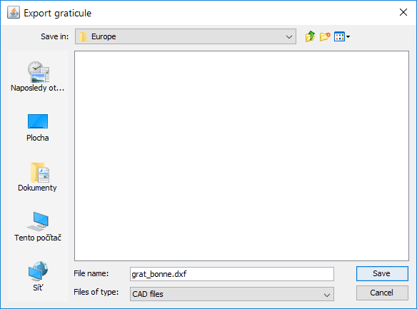
- Click on the Save button proceeds the export.
Command-line version of detectproj in C++
The generic C++ version (C++11 support) of the software detectprojv2j is available from git repository.
The basic parameters can be set using the command-line.
All methods and optimization techniques are involved.
Supported compilers: g++, msvc2015.
Basic usage
Set method, test and reference files, detection/optimization methods. Available methods: nlsm7, nlsm8, nmm7, nmm8, dem7, dem8:
| Method | Amount of parameters | Optimization | Description |
| nlsm7 | 7 | Local | Non-linear least squares optimization based on hybrid BFGS. |
| nlsm8 | 8 | Local | Non-linear least squares optimization based on hybrid BFGS, map rotation involved. |
| nmm7 | 7 | Global | Nelder-Mead optimization (Simplex method). |
| nmm8 | 8 | Global | Nelder-Mead optimization (Simplex method), map rotation involved. |
| dem7 | 7 | Global | Differential evolution optimization. |
| dem8 | 8 | Global | Differential evolution optimization, map rotation involved. |
Example:
detectprojv2 +met=nlsm7 e:\maps\Seutter\test.txt e:\maps\Seutter\reference.txt
detectprojv2 +met=nmm7 e:\maps\Seutter\test.txt e:\maps\Seutter\reference.txt
Set meridian/parallel increment
Set method, test and reference files, detection/optimization methods, meridian/parallel increments. This option is important for the DXF files with the generated graticule for setting dlat/dlon increments of meridians/parallels.
| Parameter | Default | Description |
| dlat | 10 | Latitude step between two adjacent parallels. |
| dlon | 10 | Longitude step between two adjacent meridians. |
Example:
detectprojv2 +met=nlsm7 +dlat=15 +dlon=30 e:\maps\Seutter\test.txt e:\maps\Seutter\reference.txt
Set amount of exported graticules
Set method, test and reference files, detection/optimization methods, meridian/parallel increments, amount of generated graticules exported to the DXF format.
| Parameter | Default | Desciption |
| gr | 20 | Amount of best-fit graticules exported to the DXF file; gr<=90. |
Example:
detectprojv2 +met=nlsm7 +dlat=15 +dlon=30 +gr=30 e:\maps\Seutter\test.txt e:\maps\Seutter\reference.txt